install.packages("forecast")Installing package into ‘/home/coco/R/x86_64-pc-linux-gnu-library/4.2’
(as ‘lib’ is unspecified)
Warning message in install.packages("forecast"):
“installation of package ‘forecast’ had non-zero exit status”해당 자료는 전북대학교 이영미 교수님 2023고급시계열분석 자료임
install.packages("forecast")Installing package into ‘/home/coco/R/x86_64-pc-linux-gnu-library/4.2’
(as ‘lib’ is unspecified)
Warning message in install.packages("forecast"):
“installation of package ‘forecast’ had non-zero exit status”############## package
library(forecast) #ses
library(data.table)
library(ggplot2)
library(lmtest) #dwtest
library(TTR) #SMARegistered S3 method overwritten by 'quantmod':
method from
as.zoo.data.frame zoo
Loading required package: zoo
Attaching package: ‘zoo’
The following objects are masked from ‘package:base’:
as.Date, as.Date.numeric
자꾸 forecast 설치가 안되넹
options(repr.plot.width = 15, repr.plot.height = 8)kings=scan("http://robjhyndman.com/tsdldata/misc/kings.dat",skip=3)kingskingstimeseries = ts(kings)
plot(kingstimeseries, lwd=2)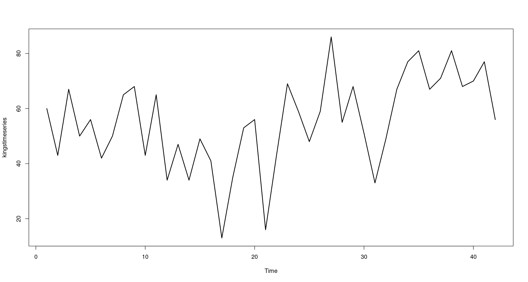
kingstimeseriesSMA(kings, n=3)n=3이므로 첫번째, 두번째에서는 값을 알 수가 없다.
56.6666666666667 = (60+43+67)/3
꼭 ts로 필수적으로 바꿀 필요는 없다.
class(SMA(kings, n=3))## window=3
kingstimeseriesSMA3 <- SMA(kingstimeseries,n=3)
plot.ts(kingstimeseries, lwd=2)
lines(kingstimeseriesSMA3, col='red', lty=2, lwd=2)
legend("topleft",
legend=c("original", expression(m==3)),
col=c("black","red"),
lty=c(1,2), lwd=2)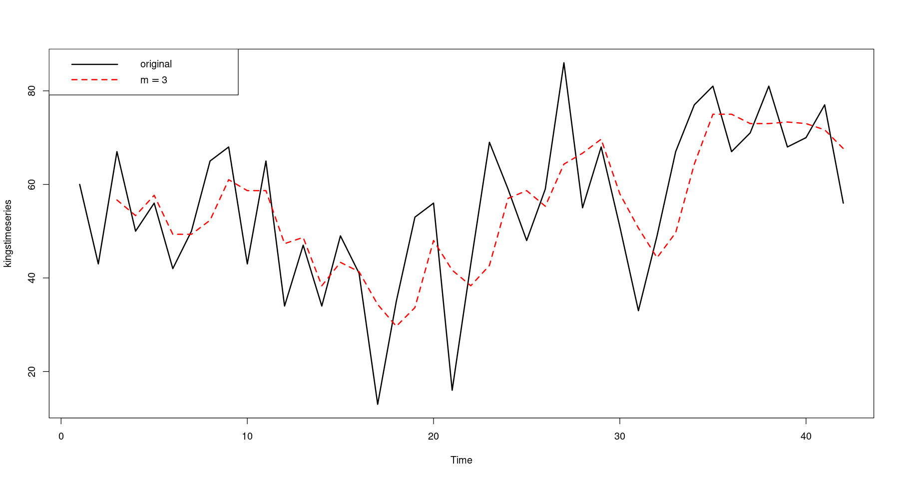
kingstimeserieskingstimeseriesSMA3## window=3 vs. 10
plot.ts(kingstimeseries, lwd=2)
lines(kingstimeseriesSMA3, col='red', lty=2, lwd=2)
lines( SMA(kingstimeseries,n=10), col='blue', lty=2, lwd=2)
legend("topleft",
legend=c("original", expression(m==3), expression(m==10)),
col=c("black","red","blue"),
lty=c(1,2,2), lwd=2)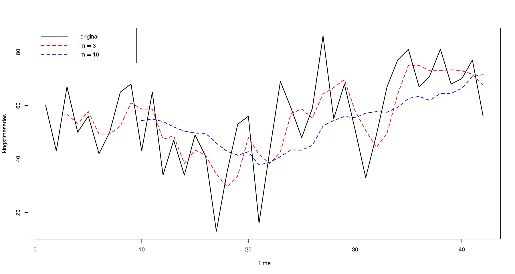
length(kings)## m=3
mean((kings[-1]- kingstimeseriesSMA3[-42])^2, na.rm=T) ##MSE : e_t(1)= z_{t+1} - hat z_t, t=3,4,...
mean(abs(kings[-1]- kingstimeseriesSMA3[-42]), na.rm=T) ##MAE
mean(abs(kings[-1]- kingstimeseriesSMA3[-42])/kings[-1], na.rm=T)*100 ##MAPEna.rm=T : 결측치는 제외하고
## m=10
mean((kings[-1]- SMA(kingstimeseries,n=10)[-42])^2, na.rm=T) ##MSE
mean(abs(kings[-1]- SMA(kingstimeseries,n=10)[-42]), na.rm=T) ##MAE
mean(abs(kings[-1]- SMA(kingstimeseries,n=10)[-42])/kings[-1], na.rm=T)*100 ##MAPE## m=4
mean((kings[-1]- SMA(kingstimeseries,n=4)[-42])^2, na.rm=T) ##MSE
mean(abs(kings[-1]- SMA(kingstimeseries,n=4)[-42]), na.rm=T) ##MAE
mean(abs(kings[-1]- SMA(kingstimeseries,n=4)[-42])/kings[-1], na.rm=T)*100 ##MAPEz <- scan("mindex.txt")
mindex <- ts(z, start = c(1986, 1), frequency = 12)
mindex| Jan | Feb | Mar | Apr | May | Jun | Jul | Aug | Sep | Oct | Nov | Dec | |
|---|---|---|---|---|---|---|---|---|---|---|---|---|
| 1986 | 9.3 | 10.7 | 13.3 | 14.1 | 17.8 | 18.1 | 19.4 | 18.8 | 19.1 | 18.4 | 18.0 | 17.0 |
| 1987 | 19.5 | 20.1 | 19.4 | 15.7 | 15.6 | 16.1 | 14.9 | 16.0 | 14.6 | 18.3 | 18.2 | 23.0 |
| 1988 | 22.2 | 22.1 | 18.8 | 17.7 | 13.8 | 12.7 | 16.5 | 15.6 | 16.3 | 10.7 | 10.4 | 7.0 |
| 1989 | 4.7 | 4.5 | 4.0 | 6.0 | 6.2 | 5.7 | 4.4 | 4.2 | 5.0 | 5.8 | 6.4 | 4.9 |
| 1990 | 7.9 | 8.2 | 11.8 | 10.0 | 11.1 | 11.7 | 12.4 | 15.2 | 14.0 | 15.2 | 12.9 | 18.0 |
| 1991 | 14.4 | 12.7 | 8.3 | 11.5 | 11.9 | 11.6 | 10.3 | 8.5 | 11.6 | 12.3 | 14.5 | 11.1 |
| 1992 | 11.8 | 12.4 | 12.7 | 9.8 | 10.0 | 10.2 | 9.6 | 6.9 | 5.3 | 4.8 | 4.6 | 1.9 |
| 1993 | 3.8 | 4.7 | 7.7 | 7.0 | 7.2 | 7.8 | 8.6 | 11.4 | 10.7 | 11.8 | 11.3 | 16.0 |
| 1994 | 13.2 | 12.0 | 8.5 | 11.4 |
mindex_sma3 <- SMA(mindex,n=3)
mindex_sma10 <- SMA(mindex,n=10)plot.ts(mindex, lwd=2)
lines(mindex_sma3, col='red', lty=2, lwd=2)
lines(mindex_sma10, col='blue', lty=2, lwd=2)
legend("topright",
legend=c("original", expression(m==3), expression(m==10)),
col=c("black","red","blue"),
lty=c(1,2,2), lwd=2)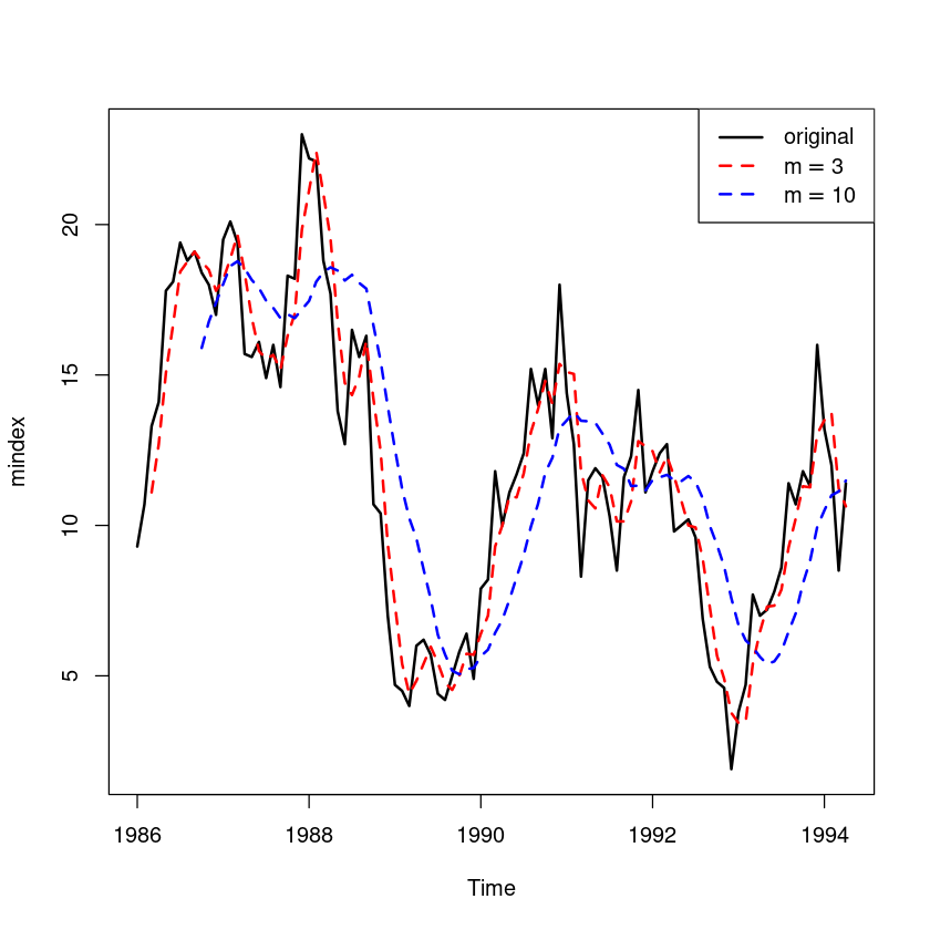
z <- scan("depart.txt")
mindex <- ts(z, start = c(1986, 1), frequency = 12)
mindex| Jan | Feb | Mar | Apr | May | Jun | Jul | Aug | Sep | Oct | Nov | Dec | |
|---|---|---|---|---|---|---|---|---|---|---|---|---|
| 1986 | 423 | 458 | 607 | 564 | 536 | 536 | 804 | 540 | 488 | 627 | 672 | 1447 |
| 1987 | 514 | 518 | 699 | 654 | 612 | 612 | 884 | 605 | 547 | 705 | 698 | 1555 |
| 1988 | 561 | 564 | 773 | 717 | 665 | 667 | 994 | 661 | 616 | 786 | 806 | 1754 |
| 1989 | 622 | 636 | 874 | 831 | 769 | 779 | 1142 | 764 | 718 | 930 | 943 | 2039 |
| 1990 | 736 | 752 | 1057 | 947 | 868 | 931 | 1311 | 896 | 867 | 1073 | 1069 | 2333 |
mindex_sma3 <- SMA(mindex,n=3)
mindex_sma12 <- SMA(mindex,n=12)plot.ts(mindex, lwd=2)
lines(mindex_sma3, col='red', lty=2, lwd=2)
lines(mindex_sma12, col='blue', lty=2, lwd=2)
legend("topright",
legend=c("original", expression(m==3), expression(m==12)),
col=c("black","red","blue"),
lty=c(1,2,2), lwd=2)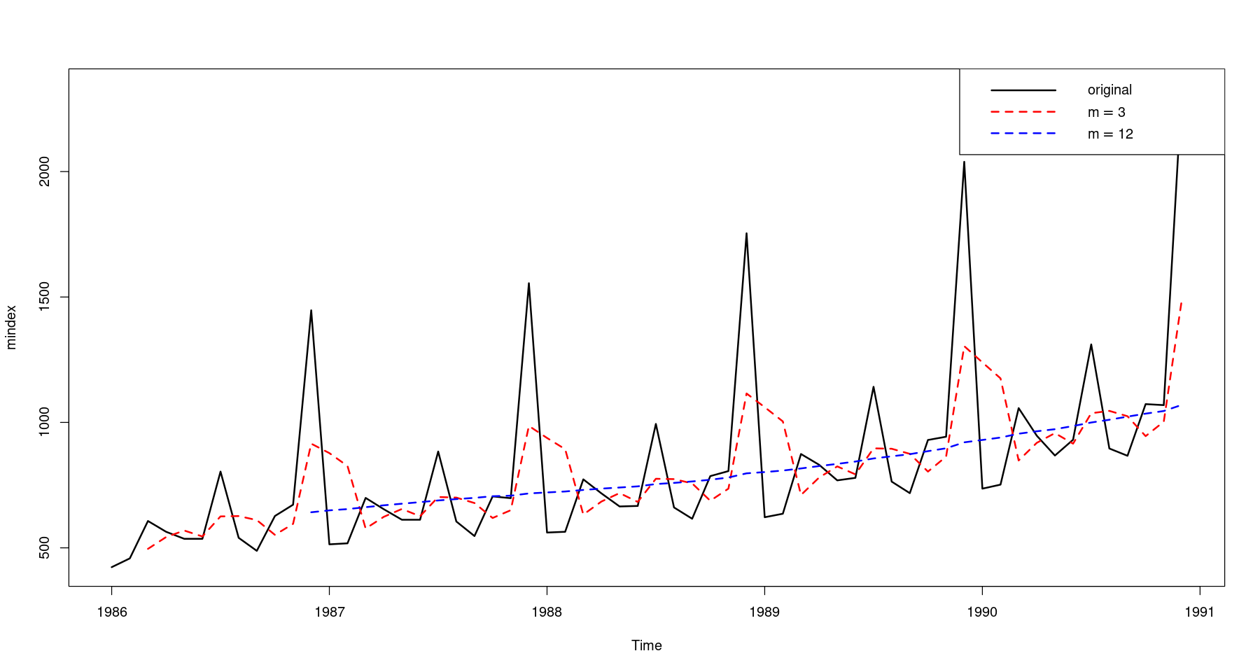
plot.ts(mindex-mindex_sma12)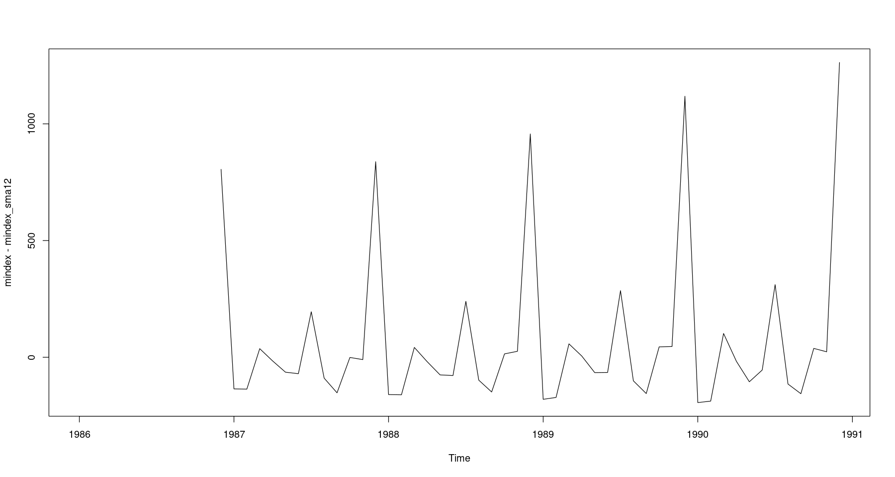
z <- scan("mindex.txt")
mindex <- ts(z, start = c(1986, 1), frequency = 12)
tmp.dat <- data.frame(day = seq.Date(as.Date("1986-01-01"),
by='month',
length.out=length(z)),
ind = z)
head(tmp.dat)
| day | ind | |
|---|---|---|
| <date> | <dbl> | |
| 1 | 1986-01-01 | 9.3 |
| 2 | 1986-02-01 | 10.7 |
| 3 | 1986-03-01 | 13.3 |
| 4 | 1986-04-01 | 14.1 |
| 5 | 1986-05-01 | 17.8 |
| 6 | 1986-06-01 | 18.1 |
ggplot(tmp.dat, aes(day, ind))+geom_line(col='skyblue', lwd=2) +
 geom_point(col='steelblue', cex=2)+
 ggtitle("중간재 출하지수")+
 theme_bw()+
 theme(plot.title = element_text(size=30),
 axis.title = element_blank())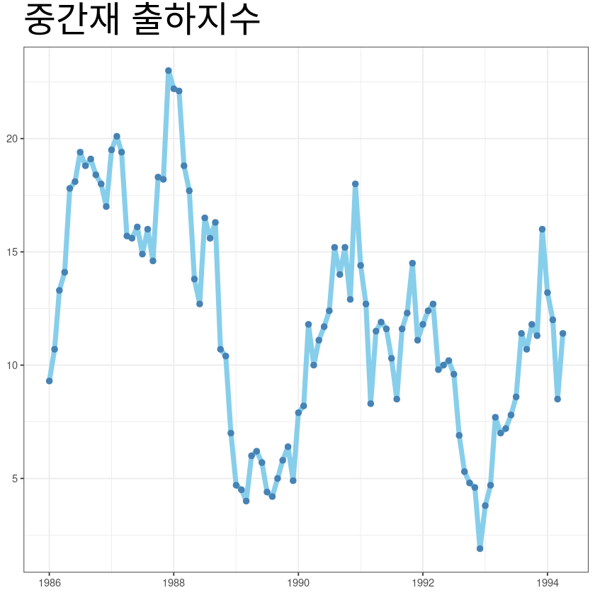
plot(mindex)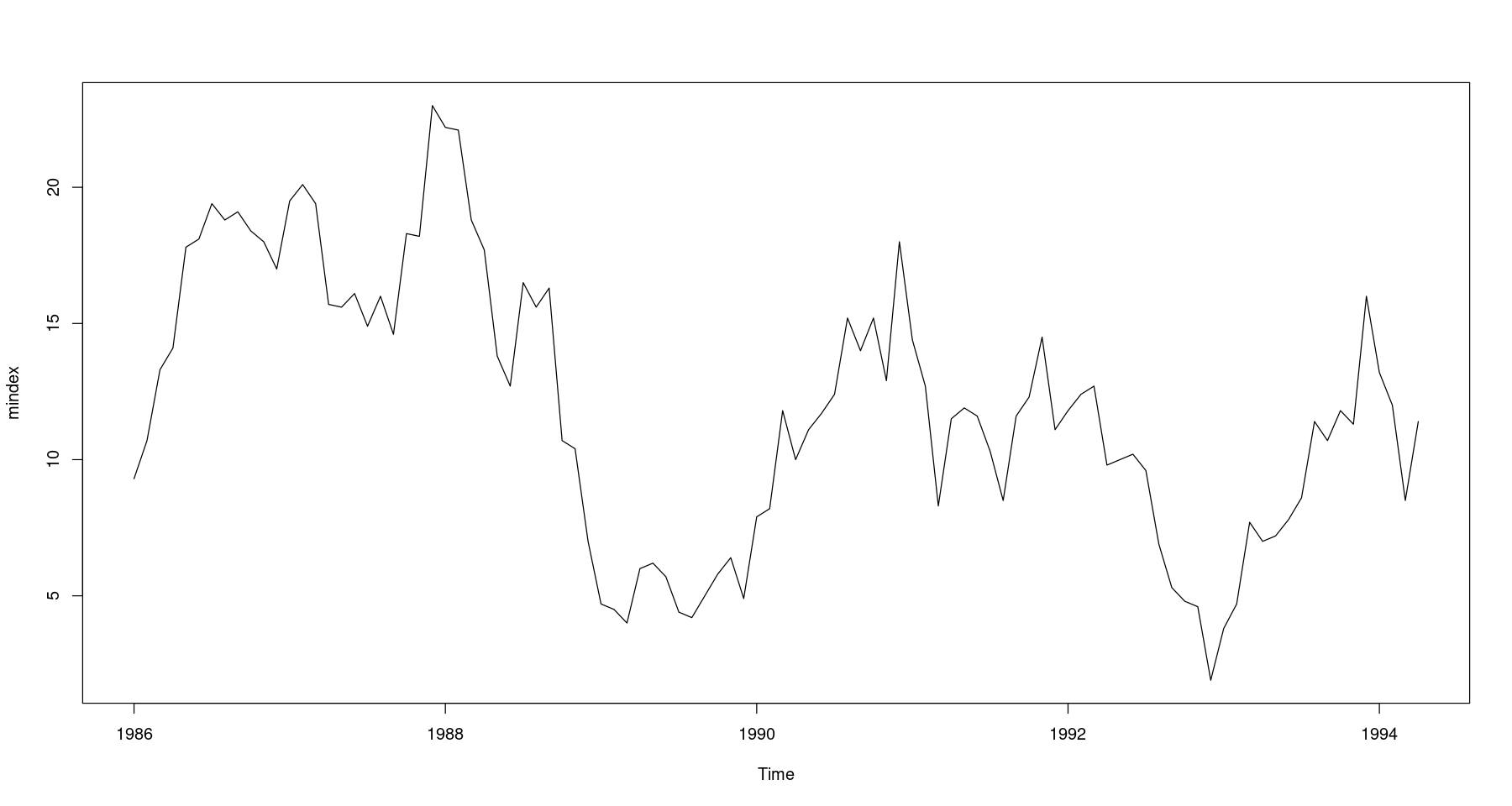
- 평활상수
alpha: level
beta: 기울기
gamma: 계절
- 평활 초기값
아래 내용 살펴보자
단순지수평활에서는 초기값을 x[1]값 을 사용함
?HoltWinters| HoltWinters {stats} | R Documentation |
Computes Holt-Winters Filtering of a given time series. Unknown parameters are determined by minimizing the squared prediction error.
HoltWinters(x, alpha = NULL, beta = NULL, gamma = NULL,
            seasonal = c("additive", "multiplicative"),
            start.periods = 2, l.start = NULL, b.start = NULL,
            s.start = NULL,
            optim.start = c(alpha = 0.3, beta = 0.1, gamma = 0.1),
optim.control = list())x |
An object of class |
alpha |
|
beta |
|
gamma |
|
seasonal |
Character string to select an |
start.periods |
Start periods used in the autodetection of start values. Must be at least 2. |
l.start |
Start value for level (a[0]). |
b.start |
Start value for trend (b[0]). |
s.start |
Vector of start values for the seasonal component ( |
optim.start |
Vector with named components |
optim.control |
Optional list with additional control parameters passed to |
The additive Holt-Winters prediction function (for time series with period length p) is
\hat Y[t+h] = a[t] + h b[t] + s[t - p + 1 + (h - 1) \bmod p],
where a[t], b[t] and s[t] are given by
a[t] = \alpha (Y[t] - s[t-p]) + (1-\alpha) (a[t-1] + b[t-1])
b[t] = \beta (a[t] -a[t-1]) + (1-\beta) b[t-1]
s[t] = \gamma (Y[t] - a[t]) + (1-\gamma) s[t-p]
The multiplicative Holt-Winters prediction function (for time series with period length p) is
\hat Y[t+h] = (a[t] + h b[t]) \times s[t - p + 1 + (h - 1) \bmod p].
where a[t], b[t] and s[t] are given by
a[t] = \alpha (Y[t] / s[t-p]) + (1-\alpha) (a[t-1] + b[t-1])
b[t] = \beta (a[t] - a[t-1]) + (1-\beta) b[t-1]
s[t] = \gamma (Y[t] / a[t]) + (1-\gamma) s[t-p]
The data in x are required to be non-zero for a multiplicative model, but it makes most sense if they are all positive.
The function tries to find the optimal values of \alpha and/or \beta and/or \gamma by minimizing the squared one-step prediction error if they are NULL (the default). optimize will be used for the single-parameter case, and optim otherwise.
For seasonal models, start values for a, b and s are inferred by performing a simple decomposition in trend and seasonal component using moving averages (see function decompose) on the start.periods first periods (a simple linear regression on the trend component is used for starting level and trend). For level/trend-models (no seasonal component), start values for a and b are x[2] and x[2] - x[1], respectively. For level-only models (ordinary exponential smoothing), the start value for a is x[1].
An object of class "HoltWinters", a list with components:
fitted |
A multiple time series with one column for the filtered series as well as for the level, trend and seasonal components, estimated contemporaneously (that is at time t and not at the end of the series). |
x |
The original series |
alpha |
alpha used for filtering |
beta |
beta used for filtering |
gamma |
gamma used for filtering |
coefficients |
A vector with named components |
seasonal |
The specified |
SSE |
The final sum of squared errors achieved in optimizing |
call |
The call used |
David Meyer David.Meyer@wu.ac.at
C. C. Holt (1957) Forecasting seasonals and trends by exponentially weighted moving averages, ONR Research Memorandum, Carnegie Institute of Technology 52. (reprint at doi:10.1016/j.ijforecast.2003.09.015).
P. R. Winters (1960). Forecasting sales by exponentially weighted moving averages. Management Science, 6, 324–342. doi:10.1287/mnsc.6.3.324.
predict.HoltWinters, optim.
require(graphics)

## Seasonal Holt-Winters
(m <- HoltWinters(co2))
plot(m)
plot(fitted(m))

(m <- HoltWinters(AirPassengers, seasonal = "mult"))
plot(m)

## Non-Seasonal Holt-Winters
x <- uspop + rnorm(uspop, sd = 5)
m <- HoltWinters(x, gamma = FALSE)
plot(m)

## Exponential Smoothing
m2 <- HoltWinters(x, gamma = FALSE, beta = FALSE)
lines(fitted(m2)[,1], col = 3)
fit0 <- HoltWinters(mindex,
                    alpha=0.3,
                    beta=FALSE,
gamma=FALSE)fit0Holt-Winters exponential smoothing without trend and without seasonal component.
Call:
HoltWinters(x = mindex, alpha = 0.3, beta = FALSE, gamma = FALSE)
Smoothing parameters:
alpha: 0.3
beta : FALSE
gamma: FALSE
Coefficients:
[,1]
a 11.2236coefficeints: 마지막 관측값(평활값)에 대한 값이 예측값이 되는것.
예측갱신
\[S_n^{(1)} = w Z_n + (1-w) S_{n-1}^{(1)}\]
tail(fit0$fitted)| xhat | level | |
|---|---|---|
| Nov 1993 | 9.97951 | 9.97951 |
| Dec 1993 | 10.37566 | 10.37566 |
| Jan 1994 | 12.06296 | 12.06296 |
| Feb 1994 | 12.40407 | 12.40407 |
| Mar 1994 | 12.28285 | 12.28285 |
| Apr 1994 | 11.14800 | 11.14800 |
coefficients: 11.14800 마지막 평활값
ls(fit0)head(fit0$fitted) ## 평활값| xhat | level | |
|---|---|---|
| Feb 1986 | 9.30000 | 9.30000 |
| Mar 1986 | 9.72000 | 9.72000 |
| Apr 1986 | 10.79400 | 10.79400 |
| May 1986 | 11.78580 | 11.78580 |
| Jun 1986 | 13.59006 | 13.59006 |
| Jul 1986 | 14.94304 | 14.94304 |
head(cbind(fit0$fitted, mindex))| fit0$fitted.xhat | fit0$fitted.level | mindex | |
|---|---|---|---|
| Jan 1986 | NA | NA | 9.3 |
| Feb 1986 | 9.30000 | 9.30000 | 10.7 |
| Mar 1986 | 9.72000 | 9.72000 | 13.3 |
| Apr 1986 | 10.79400 | 10.79400 | 14.1 |
| May 1986 | 11.78580 | 11.78580 | 17.8 |
| Jun 1986 | 13.59006 | 13.59006 | 18.1 |
관측 값이 쌓여야 해 ~
단순지수평활통계량
\[S_n^{(1)} = w \sum_{j=0}^{n-1} (1-w)^j Z_{n-j} + (1-w)^n S_0^{(1)}\]
\(S_2^{(1)} = w Z_2 + (1-w) S_0^{(1)}\)
0.3*10.7 + 0.7*9.3\(S_3^{(1)} = w Z_3 + w (1-w) Z_2 + (1-w)^2 S_0^{(1)}\)
0.3*13.3 + 0.3*0.7*10.7 + 0.7*0.7*9.3fit0$SSEplot(fit0, lwd=3, cex.main = 2)
legend("topright", legend=c("observed", "ses"), lty=1,lwd=c(1,3), col=1:2)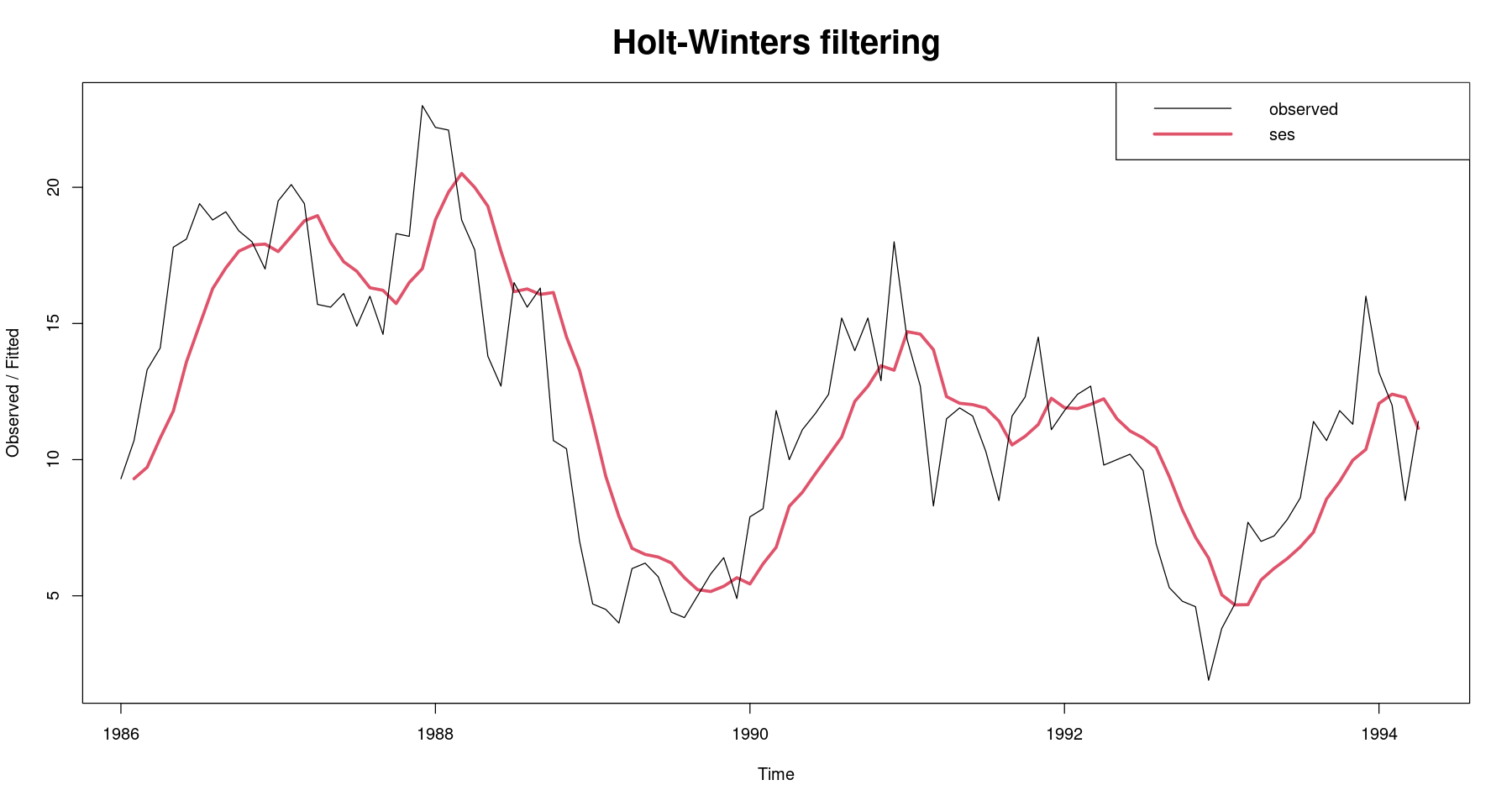
fit01 <- ses(mindex,
 alpha = 0.3,
 initial = 'simple',
h = 10) ##Exponential smoothing forecastsses: 단순지수평활만 가능한 함수
h: 마지막 데이터 이후 앞으로 예측하고 싶은 구간
fit01 Point Forecast Lo 80 Hi 80 Lo 95 Hi 95
May 1994 11.2236 7.614786 14.83241 5.704397 16.74280
Jun 1994 11.2236 7.455888 14.99131 5.461383 16.98581
Jul 1994 11.2236 7.303425 15.14377 5.228212 17.21898
Aug 1994 11.2236 7.156674 15.29052 5.003775 17.44342
Sep 1994 11.2236 7.015037 15.43216 4.787159 17.66003
Oct 1994 11.2236 6.878013 15.56918 4.577601 17.86959
Nov 1994 11.2236 6.745181 15.70201 4.374450 18.07274
Dec 1994 11.2236 6.616176 15.83102 4.177155 18.27004
Jan 1995 11.2236 6.490686 15.95651 3.985235 18.46196
Feb 1995 11.2236 6.368439 16.07875 3.798273 18.64892ls(fit01)summary(fit01)
Forecast method: Simple exponential smoothing
Model Information:
Simple exponential smoothing
Call:
ses(y = mindex, h = 10, initial = "simple", alpha = 0.3)
Smoothing parameters:
alpha = 0.3
Initial states:
l = 9.3
sigma: 2.816
Error measures:
ME RMSE MAE MPE MAPE MASE ACF1
Training set 0.06411989 2.81597 2.248923 -7.657492 24.93904 0.4105067 0.6648489
Forecasts:
         Point Forecast    Lo 80    Hi 80    Lo 95    Hi 95
May 1994        11.2236 7.614786 14.83241 5.704397 16.74280
Jun 1994        11.2236 7.455888 14.99131 5.461383 16.98581
Jul 1994        11.2236 7.303425 15.14377 5.228212 17.21898
Aug 1994        11.2236 7.156674 15.29052 5.003775 17.44342
Sep 1994        11.2236 7.015037 15.43216 4.787159 17.66003
Oct 1994        11.2236 6.878013 15.56918 4.577601 17.86959
Nov 1994        11.2236 6.745181 15.70201 4.374450 18.07274
Dec 1994        11.2236 6.616176 15.83102 4.177155 18.27004
Jan 1995        11.2236 6.490686 15.95651 3.985235 18.46196
Feb 1995 11.2236 6.368439 16.07875 3.798273 18.64892tail(cbind(fit0$fitted, mindex))| fit0$fitted.xhat | fit0$fitted.level | mindex | |
|---|---|---|---|
| Nov 1993 | 9.97951 | 9.97951 | 11.3 |
| Dec 1993 | 10.37566 | 10.37566 | 16.0 |
| Jan 1994 | 12.06296 | 12.06296 | 13.2 |
| Feb 1994 | 12.40407 | 12.40407 | 12.0 |
| Mar 1994 | 12.28285 | 12.28285 | 8.5 |
| Apr 1994 | 11.14800 | 11.14800 | 11.4 |
- 예측 갱신
\[S_n^{(1)} = wZ_n + (1-w)S_{n-1}^{(1)}\]
\(S_{100}^{(1)} = w Z_{100} + (1-w) S_{(99)}^{(1)}\)
0.3*11.4+0.7*11.148000.3*11.4+0.7*11.147995summary(fit01)
Forecast method: Simple exponential smoothing

Model Information:
Simple exponential smoothing

Call:
 ses(y = mindex, h = 10, initial = "simple", alpha = 0.3)

  Smoothing parameters:
    alpha = 0.3

  Initial states:
    l = 9.3

  sigma:  2.816
Error measures:
                     ME    RMSE      MAE       MPE     MAPE      MASE      ACF1
Training set 0.06411989 2.81597 2.248923 -7.657492 24.93904 0.4105067 0.6648489

Forecasts:
         Point Forecast    Lo 80    Hi 80    Lo 95    Hi 95
May 1994        11.2236 7.614786 14.83241 5.704397 16.74280
Jun 1994        11.2236 7.455888 14.99131 5.461383 16.98581
Jul 1994        11.2236 7.303425 15.14377 5.228212 17.21898
Aug 1994        11.2236 7.156674 15.29052 5.003775 17.44342
Sep 1994        11.2236 7.015037 15.43216 4.787159 17.66003
Oct 1994        11.2236 6.878013 15.56918 4.577601 17.86959
Nov 1994        11.2236 6.745181 15.70201 4.374450 18.07274
Dec 1994        11.2236 6.616176 15.83102 4.177155 18.27004
Jan 1995        11.2236 6.490686 15.95651 3.985235 18.46196
Feb 1995 11.2236 6.368439 16.07875 3.798273 18.64892plot(fit01,, cex.main = 2)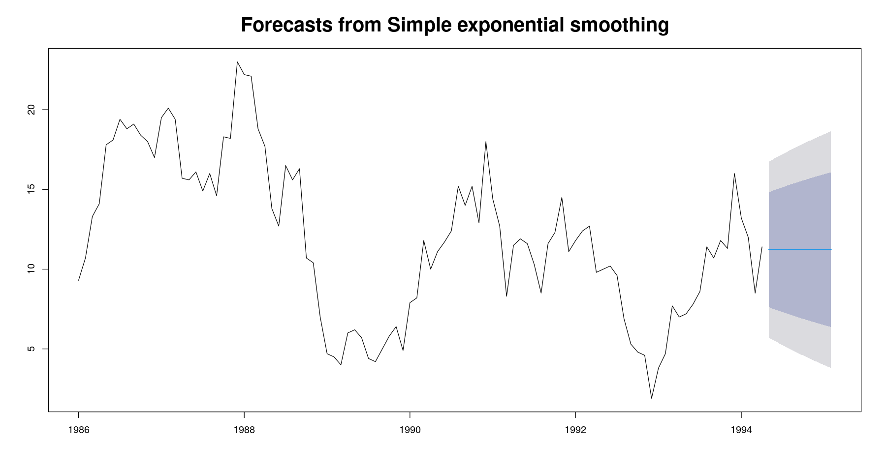
w <-c(seq(0.1,0.8,0.1), seq(0.81, 0.99, 0.01))SSE_ses <- sapply(w, function(alpha) HoltWinters(mindex,
alpha=alpha,
beta=FALSE,
gamma=FALSE)$SSE)
plot(w,SSE_ses, type="o", xlab="weight", ylab="SSE", pch=16,
main="1 시차 후 예측오차의 제곱합",
cex.main = 2, cex.lab=2)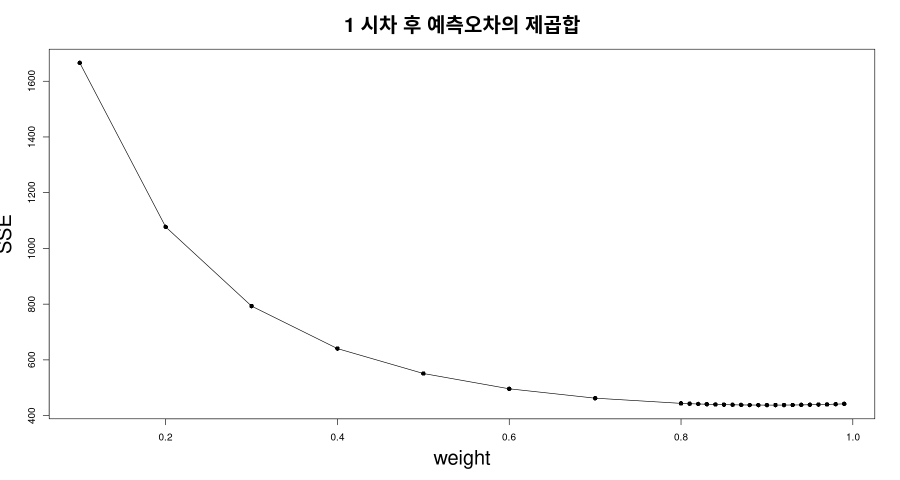
- SSE를 가장 작게 하는 값 찾자
which.min(SSE_ses)w[which.min(SSE_ses)]plot(w[-(1:7)],SSE_ses[-(1:7)], type="o", xlab="weight", ylab="SSE", pch=16,
main="1 시차 후 예측오차의 제곱합",
cex.main = 2, cex.lab=2)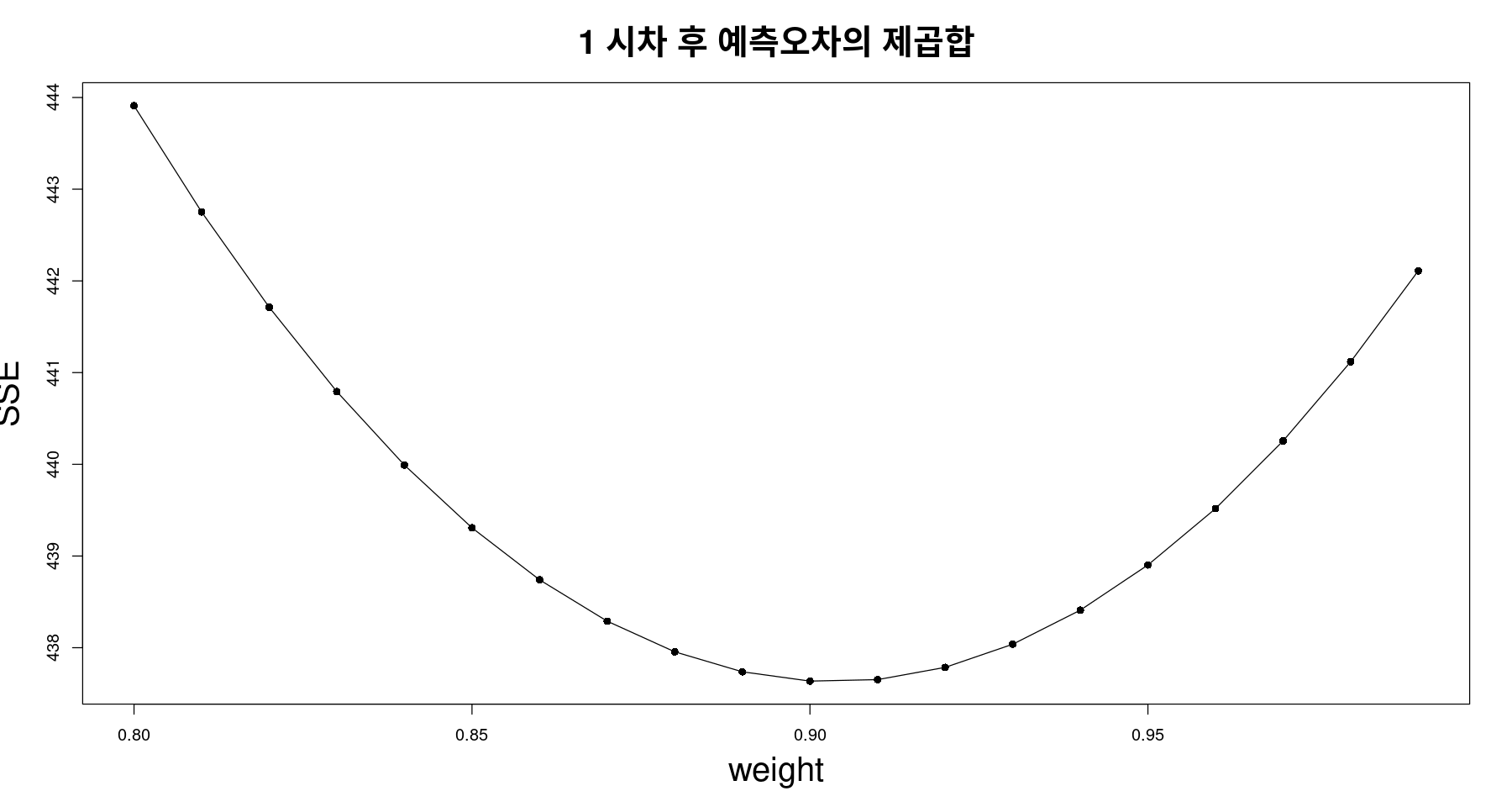
fit1 <- ses(mindex, alpha=w[which.min(SSE_ses)], initial = "simple", h=6)plot(fit1, xlab="", ylab="",
main="중간재 출하지수와 단순지수평활값 alpha=0.9",
lty=1,col="black",
cex.main = 2, cex.lab=2 )
lines(fitted(fit1), col="red", lty=2)
legend("topright", legend=c("Mindex", expression(alpha==0.9)),
lty=1:2,col=c("black","red"))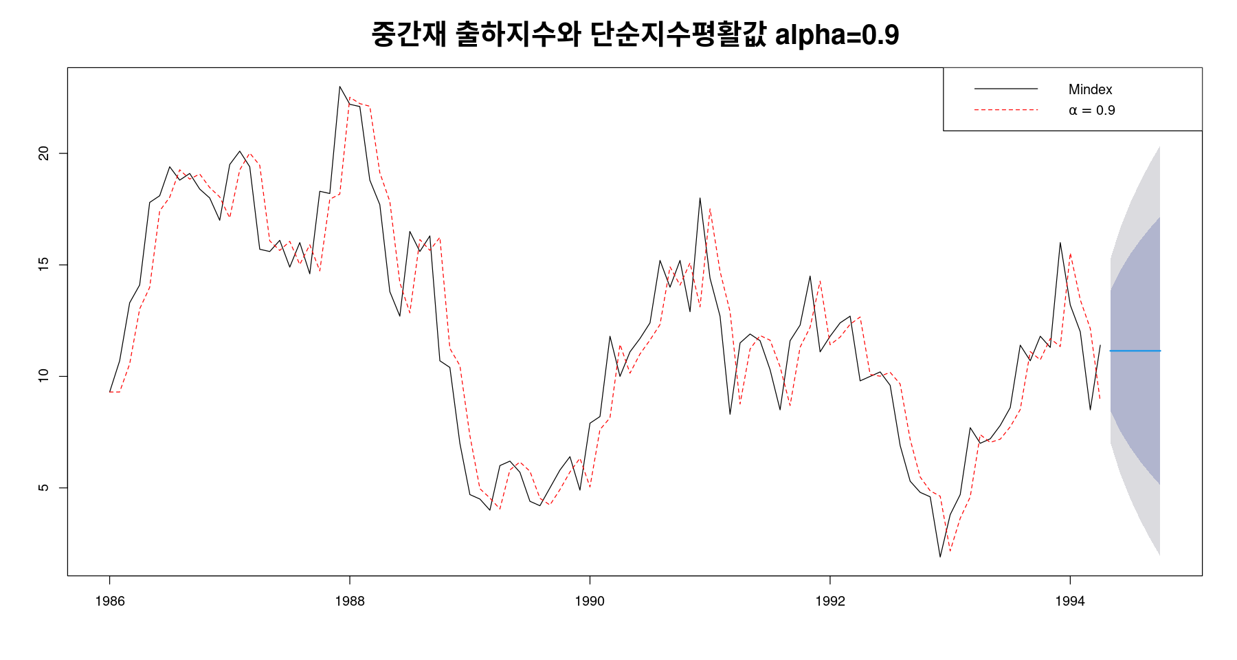
fit0_w <- HoltWinters(mindex,
 beta=FALSE,
 gamma=FALSE)
fit0_w
Holt-Winters exponential smoothing without trend and without seasonal component.
Call:
HoltWinters(x = mindex, beta = FALSE, gamma = FALSE)
Smoothing parameters:
alpha: 0.9036403
beta : FALSE
gamma: FALSE
Coefficients:
[,1]
a 11.15433fit1 <- ses(mindex, alpha=fit0_w$alpha, h=12)ls(fit1)plot(fit1$residuals, ylab="residual",
main="예측 오차의 시계열그림 : alpha=0.9",
cex.main = 2, cex.lab=2); abline(h=0)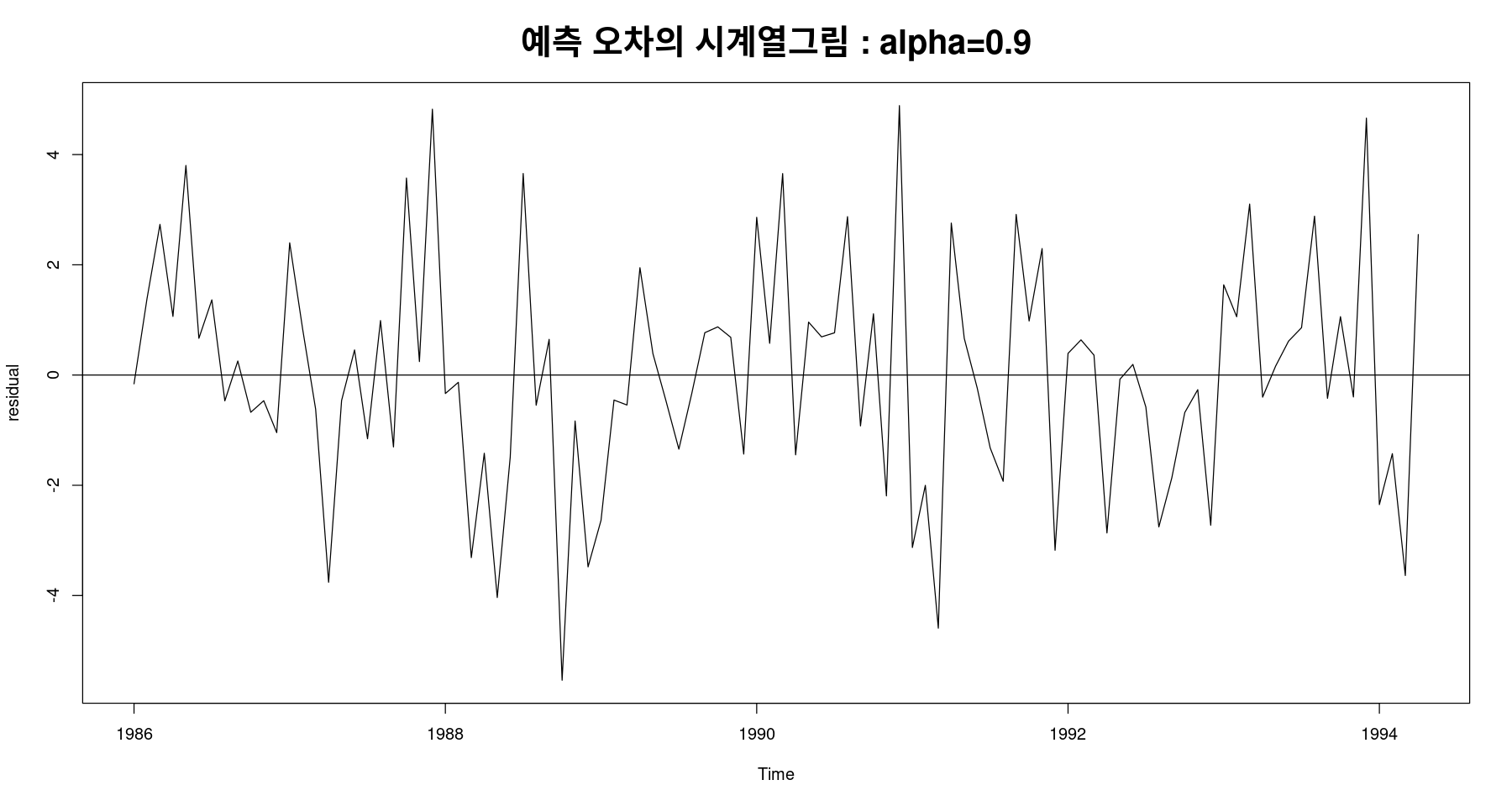
t.test(fit1$residual)
    One Sample t-test

data:  fit1$residual
t = 0.089225, df = 99, p-value = 0.9291
alternative hypothesis: true mean is not equal to 0
95 percent confidence interval:
 -0.3983934  0.4359099
sample estimates:
 mean of x
0.01875828 \(H_0\): \(\mu=0\) vs. \(H_1: \mu \neq 0\)
귀무가설을 기각할 수 없음. 평균은 0이다.
dwtest(lm(fit1$residual~1))
    Durbin-Watson test

data:  lm(fit1$residual ~ 1)
DW = 2.0244, p-value = 0.549
alternative hypothesis: true autocorrelation is greater than 0\(H_0\): 독립이다.
dwtest에는 회귀모형이 들어가야 함.
dwtest(lm(fit1$residual~1), alternative = "two.sided")
    Durbin-Watson test

data:  lm(fit1$residual ~ 1)
DW = 2.0244, p-value = 0.902
alternative hypothesis: true autocorrelation is not 0fit2 <- ses(mindex, alpha=0.3, h=6)
plot(fit2, xlab="year", ylab="mindex",
main=expression("중간재 출하지수와 단순지수평활값 "~alpha==0.3),
lty=1,col="black",
cex.main = 2,
cex.lab=2)
lines(fitted(fit2), col="red", lty=2)
legend("topright",
legend=c("Mindex",expression(alpha==0.3)),
lty=1:2,
col=c("black","red"))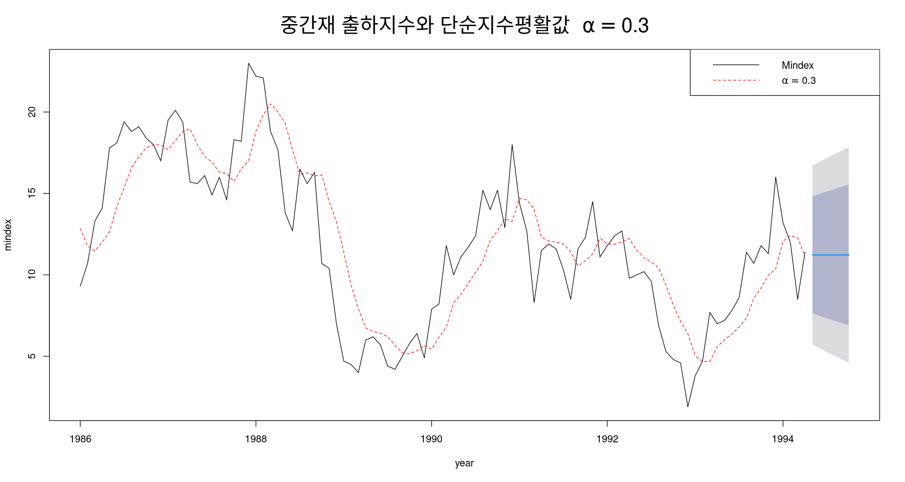
plot(fit2$residuals, ylab="residual",
 main=expression("중간재 출하지수와 단순지수평활값 "~alpha==0.3),
 cex.main = 2,
 cex.lab=2); abline(h=0)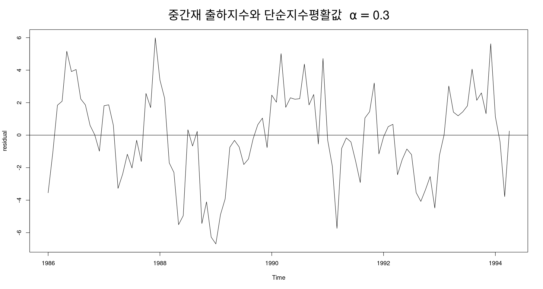
오차의 평균이 0인가?
t.test(fit2$residual)
    One Sample t-test

data:  fit2$residual
t = -0.19433, df = 99, p-value = 0.8463
alternative hypothesis: true mean is not equal to 0
95 percent confidence interval:
 -0.6067721  0.4985236
sample estimates:
  mean of x
-0.05412425
오차가 독립인가?
dwtest(lm(fit2$residual~1))
    Durbin-Watson test

data:  lm(fit2$residual ~ 1)
DW = 0.70285, p-value = 2.853e-11
alternative hypothesis: true autocorrelation is greater than 0z <- scan("stock.txt")
stock <- ts(z, start=c(1984,1), frequency=12)plot(stock, main = '월별주가지수', cex.main=2, cex.lab=2)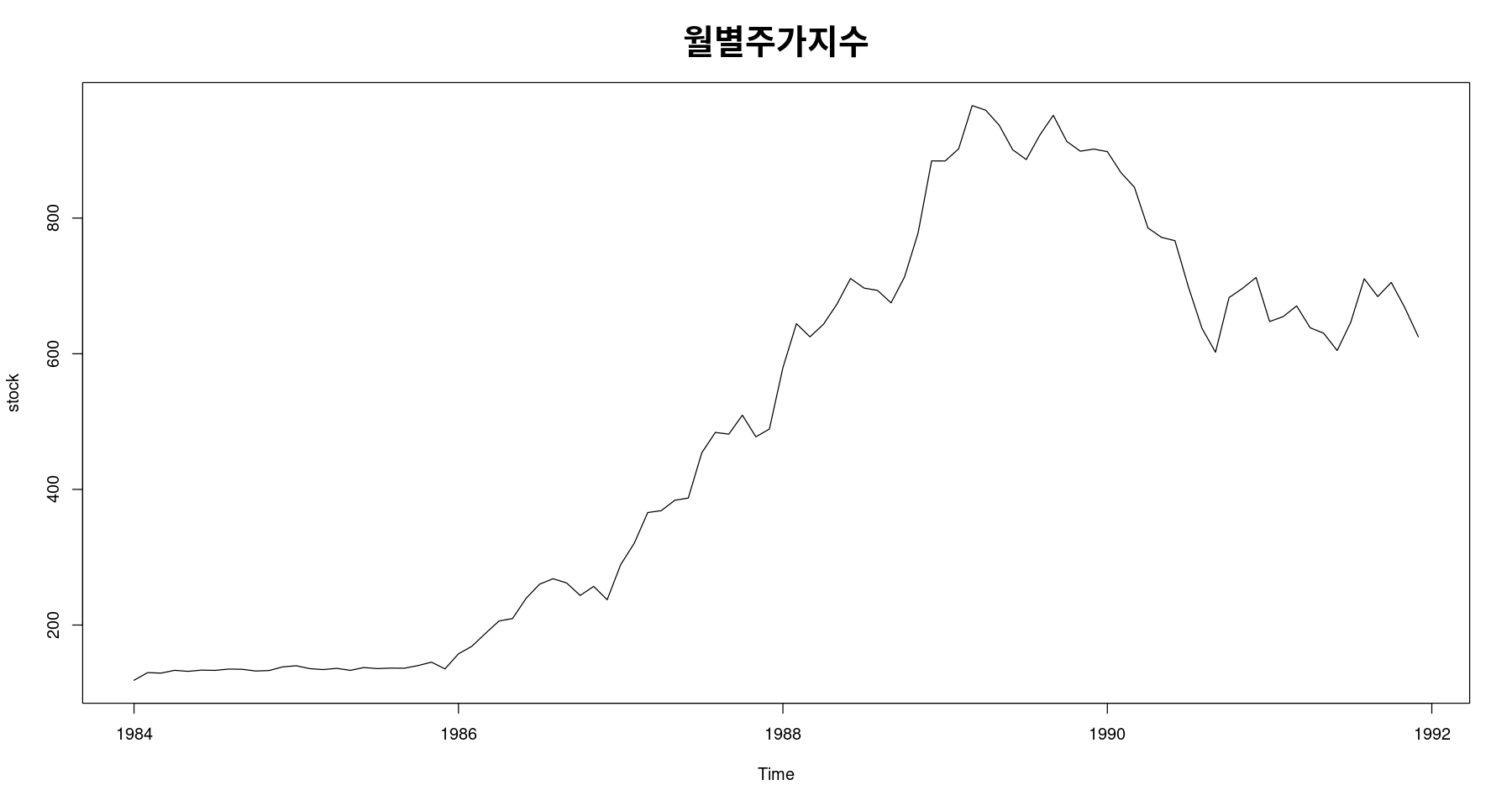
fit4 = holt(stock, alpha=0.6, beta=0.6, h=6)
fit4$model
Holt's method
Call:
holt(y = stock, h = 6, alpha = 0.6, beta = 0.6)
Smoothing parameters:
alpha = 0.6
beta = 0.6
Initial states:
l = 115.6009
b = 6.8098
sigma: 40.2546
AIC AICc BIC
1149.575 1149.836 1157.268 plot(fit4, ylab="", xlab="", lty=1, col="black",
main="주가지수와 이중지수평활값 : alpha=beta=0.6"
)
lines(fitted(fit4), col="red", lty=2)
legend("topleft", lty=1:2, col=c("black","red"), c("Index", "Double"), bty = "n")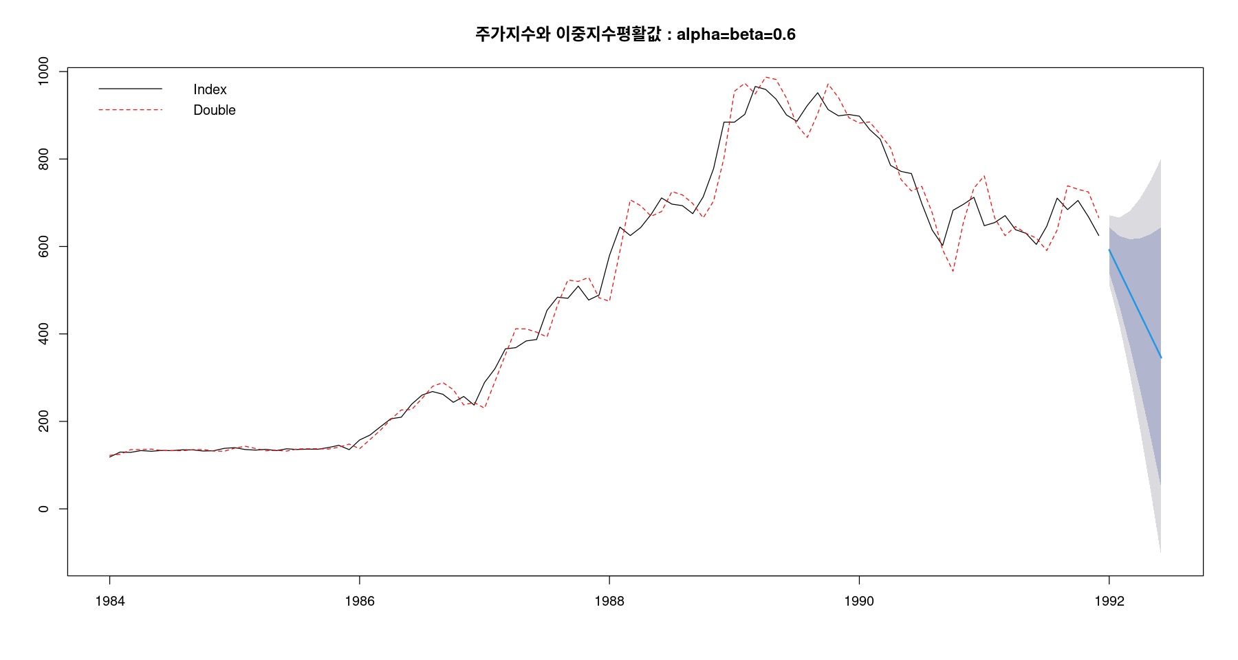
fit5 = holt(stock, h=6)
fit5$model
Holt's method
Call:
holt(y = stock, h = 6)
Smoothing parameters:
alpha = 0.9999
beta = 0.1071
Initial states:
l = 124.1137
b = 3.4954
sigma: 31.8609
AIC AICc BIC
1108.677 1109.343 1121.498 fit50 <- HoltWinters(stock,
gamma = FALSE)fit50Holt-Winters exponential smoothing with trend and without seasonal component.
Call:
HoltWinters(x = stock, gamma = FALSE)
Smoothing parameters:
alpha: 1
beta : 0.1094451
gamma: FALSE
Coefficients:
[,1]
a 625.060000
b -7.097122predict(fit50, n.ahead=12, prediction.interval = T, level=0.95) | fit | upr | lwr | |
|---|---|---|---|
| Jan 1992 | 617.9629 | 680.0626 | 555.8631 |
| Feb 1992 | 610.8658 | 703.6185 | 518.1130 |
| Mar 1992 | 603.7686 | 723.4869 | 484.0504 |
| Apr 1992 | 596.6715 | 742.0570 | 451.2860 |
| May 1992 | 589.5744 | 760.1877 | 418.9611 |
| Jun 1992 | 582.4773 | 778.2851 | 386.6695 |
| Jul 1992 | 575.3801 | 796.5695 | 354.1907 |
| Aug 1992 | 568.2830 | 815.1705 | 321.3955 |
| Sep 1992 | 561.1859 | 834.1678 | 288.2040 |
| Oct 1992 | 554.0888 | 853.6121 | 254.5655 |
| Nov 1992 | 546.9917 | 873.5358 | 220.4475 |
| Dec 1992 | 539.8945 | 893.9596 | 185.8294 |
fit5 Point Forecast Lo 80 Hi 80 Lo 95 Hi 95
Jan 1992 618.0360 577.2045 658.8674 555.5897 680.4822
Feb 1992 611.0079 550.0961 671.9196 517.8514 704.1644
Mar 1992 603.9798 525.4452 682.5144 483.8715 724.0881
Apr 1992 596.9517 501.6745 692.2290 451.2377 742.6657
May 1992 589.9237 478.2155 701.6319 419.0807 760.7666
Jun 1992 582.8956 454.7987 710.9924 386.9883 778.8028- 시점 n에서 l-시차 후의 예측값
\[\hat {Z}_n(l) = \hat {\beta}_{0,n} + \hat {\beta}_{1,n}(n+l) = \left( 2+ \dfrac{w}{1-w}l \right) S_n^{(1)} - \left( 1+ \dfrac{w}{1-w}l \right) S_n^{(2)}\]
plot(fit5, ylab="Index", xlab="year", lty=1, col="black",
 main=expression("중간재 출하지수와 이중지수평활값 : "~alpha~","~beta~ " : estimated"),
 cex.main=2)
lines(fitted(fit5), col="red", lty=2)
legend("topleft", lty=1:2, col=c("black","red"), c("Index", "Double"))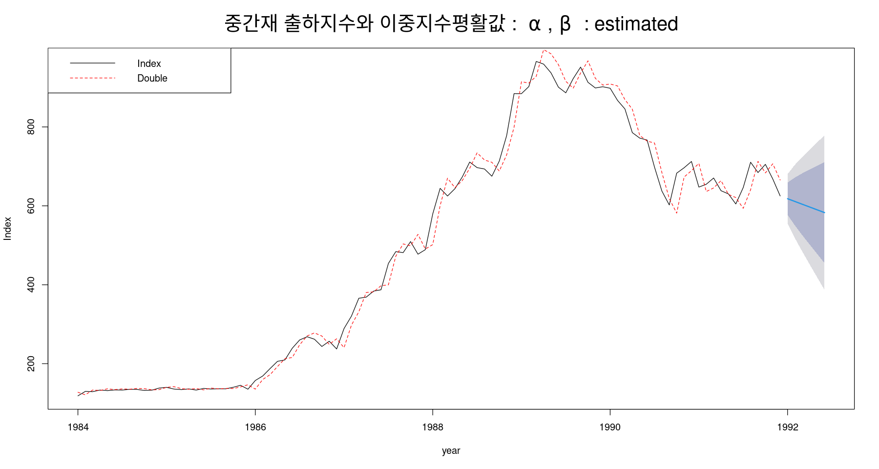
plot(resid(fit5), main=expression("Residual Plot : "~alpha~","~beta~ " : estimated"),
 cex.main=2)
abline(h=0)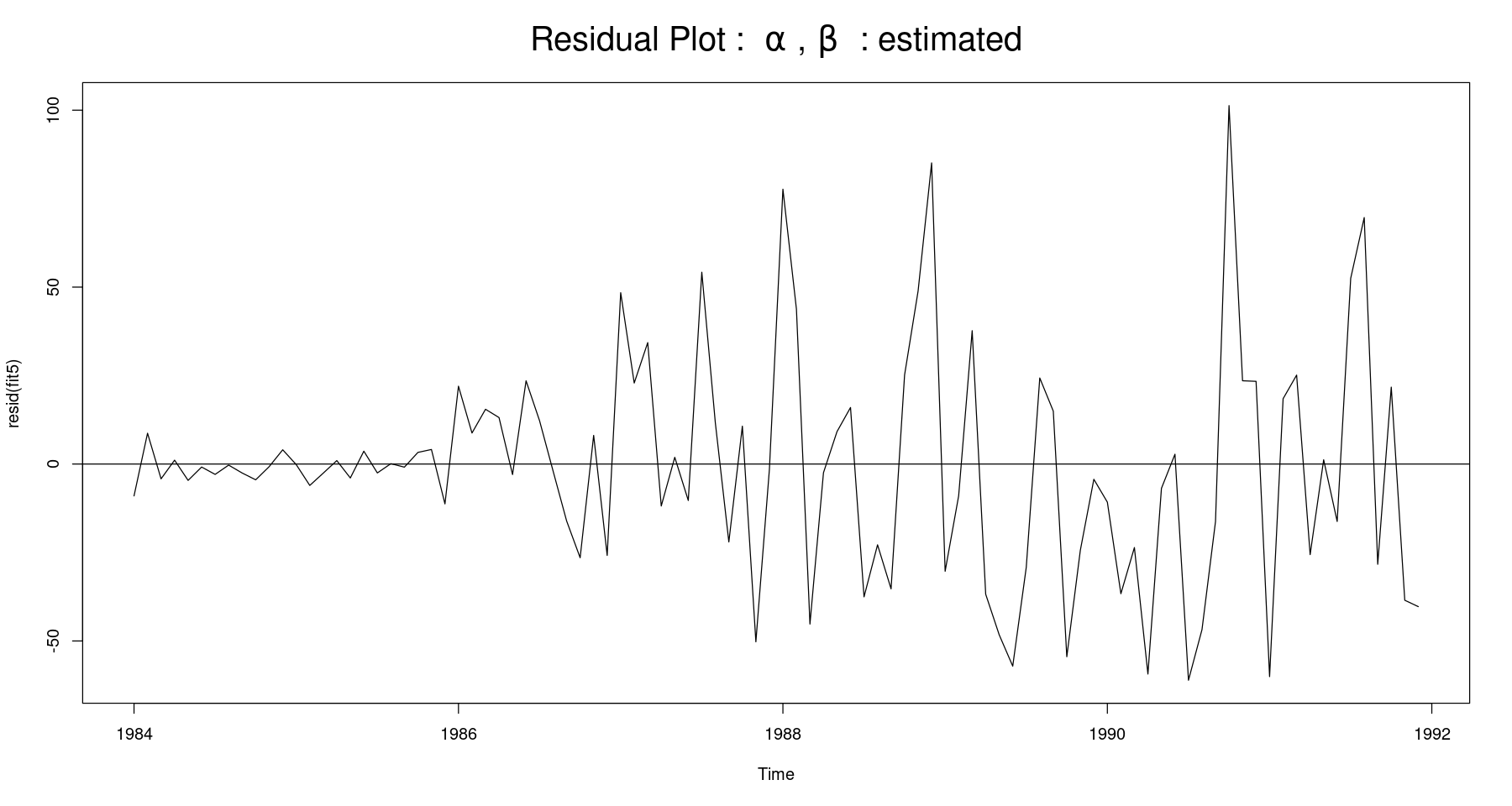
dwtest(lm(fit5$residuals~1), alternative = "two.sided")
    Durbin-Watson test

data:  lm(fit5$residuals ~ 1)
DW = 1.658, p-value = 0.09054
alternative hypothesis: true autocorrelation is not 0z <- scan("koreapass.txt")
pass <- ts(z, start=c(1981,1), frequency=12)ts에 주기가 들어가 있어야 holtwinter에서 계절을 적합할 수 있다
plot.ts(pass)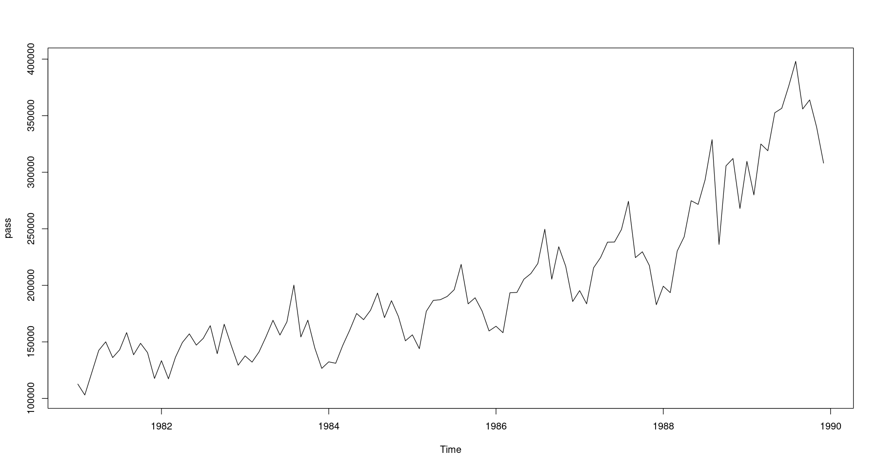
가법 모형? 승법 모형? 무엇을 쓸지 정해줘야 함
fit_hw <- HoltWinters(pass, seasonal="additive") #default는 additivefit_hwHolt-Winters exponential smoothing with trend and additive seasonal component.
Call:
HoltWinters(x = pass, seasonal = "additive")
Smoothing parameters:
alpha: 0.4810767
beta : 0.0383379
gamma: 0.7345988
Coefficients:
[,1]
a 347794.753
b 3363.251
s1 -12186.666
s2 -33643.322
s3 4855.643
s4 5000.713
s5 29085.909
s6 22953.006
s7 32200.195
s8 49687.643
s9 -11655.430
s10 10218.813
s11 -4226.391
s12 -38683.394head(fit_hw$fitted)| xhat | level | trend | season | |
|---|---|---|---|---|
| Jan 1982 | 128208.0 | 135375.1 | 769.6180 | -7936.701 |
| Feb 1982 | 114877.0 | 138637.6 | 865.1923 | -24625.868 |
| Mar 1982 | 135627.2 | 140706.0 | 911.3201 | -5990.160 |
| Apr 1982 | 149303.2 | 141945.3 | 923.8952 | 6433.924 |
| May 1982 | 156969.9 | 142952.4 | 927.0829 | 13090.465 |
| Jun 1982 | 147259.4 | 143945.4 | 929.6108 | 2384.382 |
135375.1+769.6180-7936.701xhat = level + trend + season
- 계절지수평활 예측
\[\hat{Z}_n(k) = \hat{T}_n + \hat{\beta}_{1,n}k + \hat{S}_{n+k-s}, k=1,2,\dots, s\]
plot(fit_hw, lwd=2)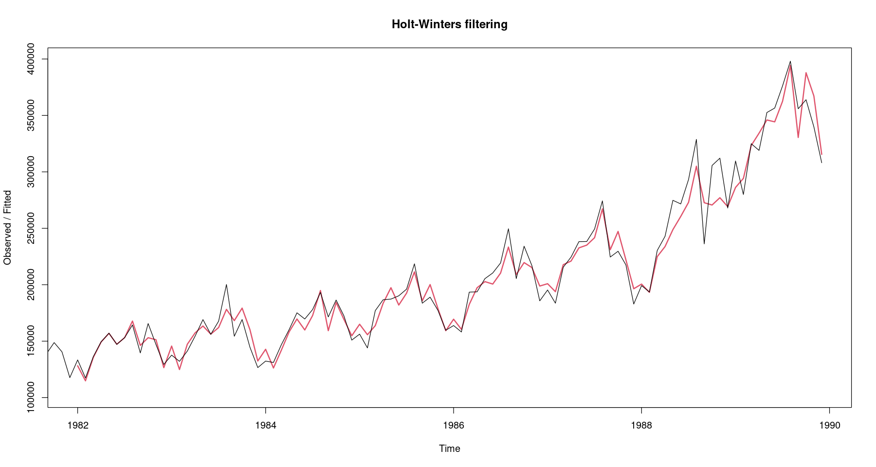
predict(fit_hw, n.ahead=12, prediction.interval = T, level=0.95)| fit | upr | lwr | |
|---|---|---|---|
| Jan 1990 | 338971.3 | 362386.4 | 315556.2 |
| Feb 1990 | 320877.9 | 347051.8 | 294704.1 |
| Mar 1990 | 362740.1 | 391587.4 | 333892.9 |
| Apr 1990 | 366248.5 | 397711.4 | 334785.5 |
| May 1990 | 393696.9 | 427736.7 | 359657.1 |
| Jun 1990 | 390927.3 | 427518.3 | 354336.2 |
| Jul 1990 | 403537.7 | 442664.2 | 364411.2 |
| Aug 1990 | 424388.4 | 466041.9 | 382734.9 |
| Sep 1990 | 366408.6 | 410586.3 | 322230.9 |
| Oct 1990 | 391646.1 | 438349.7 | 344942.5 |
| Nov 1990 | 380564.1 | 429798.8 | 331329.4 |
| Dec 1990 | 349470.4 | 401244.2 | 297696.5 |
fit6= hw(pass,
 alpha = fit_hw$alpha,
 beta = fit_hw$beta,
 gamma = fit_hw$gamma,
 seasonal="additive",
 initial="simple",
 h=12)
fit6$model
Holt-Winters' additive method
Call:
hw(y = pass, h = 12, seasonal = "additive", initial = "simple",
Call:
alpha = fit_hw$alpha, beta = fit_hw$beta, gamma = fit_hw$gamma)
Smoothing parameters:
alpha = 0.4811
beta = 0.0383
gamma = 0.7346
Initial states:
l = 134510.75
b = 874.0694
s = -16817.75 6028.25 14250.25 4115.25 23712.25 8522.25
1617.25 15553.25 7985.25 -11710.75 -31440.75 -21814.75
sigma: 12483.69fit6 Point Forecast Lo 80 Hi 80 Lo 95 Hi 95
Jan 1990 339962.9 323964.4 355961.4 315495.3 364430.4
Feb 1990 307759.0 289731.1 325786.9 280187.7 335330.3
Mar 1990 354907.1 334791.7 375022.5 324143.3 385670.9
Apr 1990 353308.1 331046.6 375569.6 319262.1 387354.2
May 1990 391666.8 367200.6 416133.1 354249.0 429084.7
Jun 1990 393291.1 366562.0 420020.2 352412.5 434169.7
Jul 1990 408050.5 379001.1 437099.9 363623.2 452477.8
Aug 1990 428126.3 396699.7 459552.8 380063.5 476189.1
Sep 1990 374195.2 340335.6 408054.7 322411.4 425978.9
Oct 1990 381277.1 344929.5 417624.7 325688.2 436866.0
Nov 1990 373366.6 334476.8 412256.5 313889.7 432843.5
Dec 1990 347593.0 306107.7 389078.3 284146.7 411039.3plot(fit6, ylab="passenger", xlab="year", lty=1, col="blue",
main="Winters 가법계절지수평활된 자료의 시계열 그림",
cex.main=2)
lines(fit6$fitted, lwd=3, col='red', lty=2)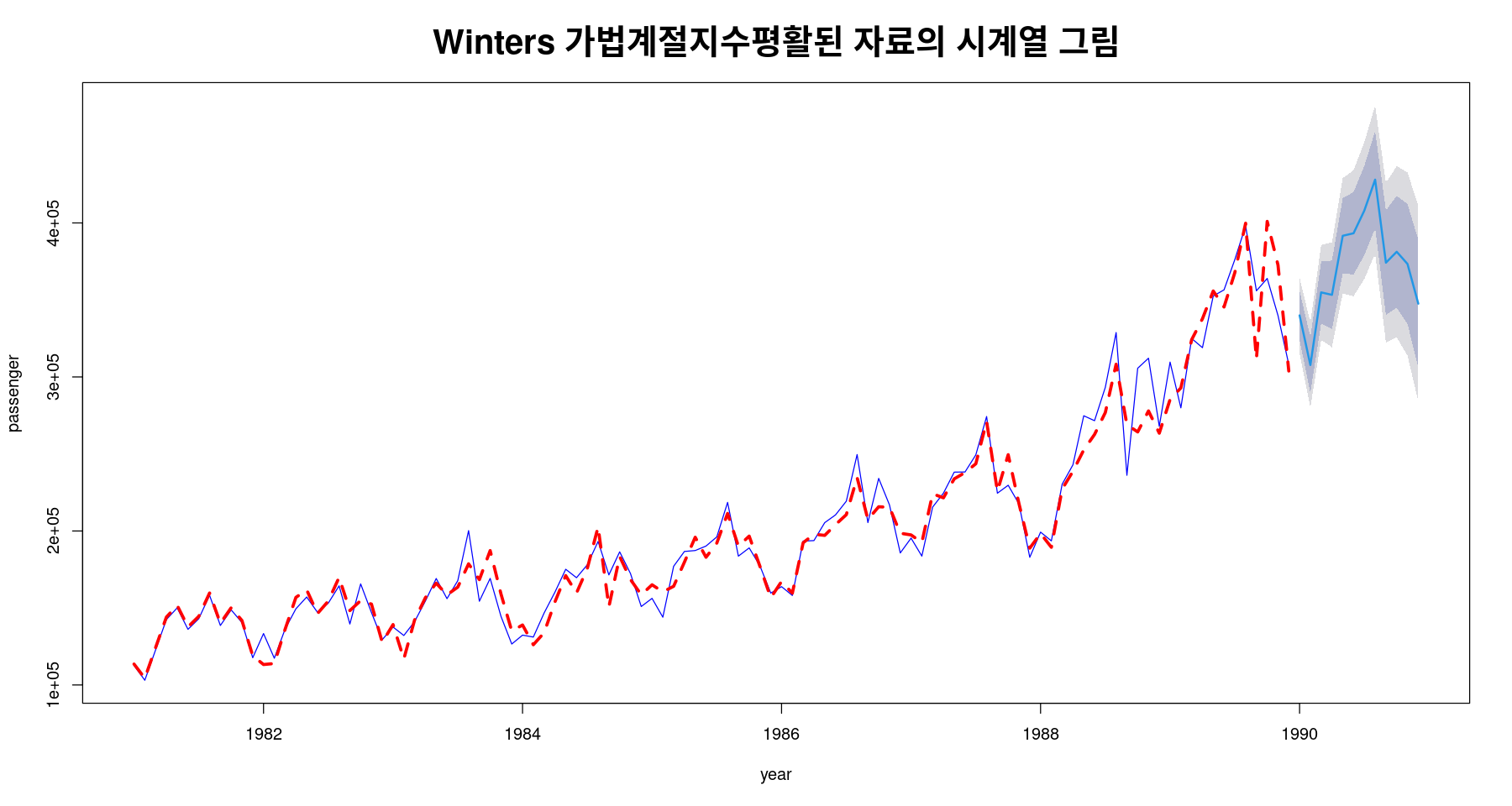
ts.plot(fit6$residual, ylab="residual",
 main="가법모형의 잔차 그림",
 cex.main=2); abline(h=0)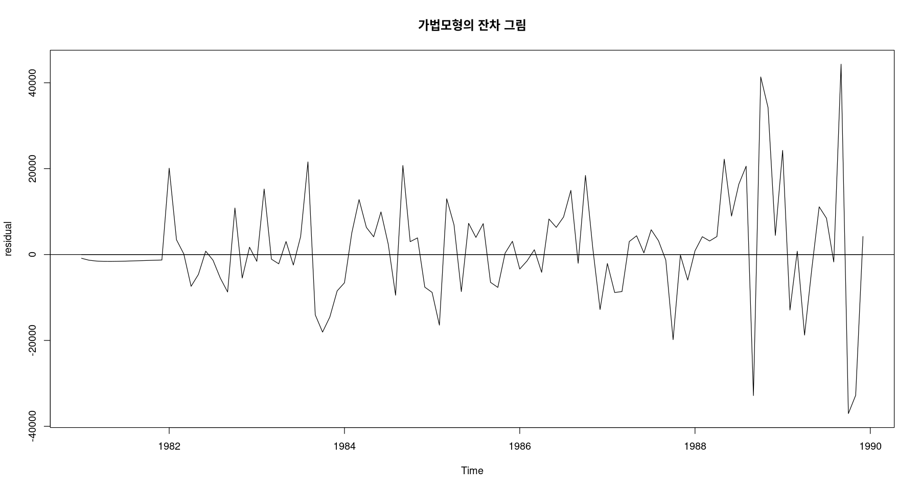
dwtest(lm(fit6$residual~1), alternative = 'two.sided')
    Durbin-Watson test

data:  lm(fit6$residual ~ 1)
DW = 1.9794, p-value = 0.9139
alternative hypothesis: true autocorrelation is not 0fit_hw_m <- HoltWinters(pass, seasonal="multiplicative")
fit_hw_mHolt-Winters exponential smoothing with trend and multiplicative seasonal component.
Call:
HoltWinters(x = pass, seasonal = "multiplicative")
Smoothing parameters:
alpha: 0.5623303
beta : 0.03452066
gamma: 0.3506508
Coefficients:
[,1]
a 3.560417e+05
b 3.517556e+03
s1 9.199511e-01
s2 8.489190e-01
s3 9.796617e-01
s4 1.016528e+00
s5 1.095078e+00
s6 1.060795e+00
s7 1.089621e+00
s8 1.178393e+00
s9 9.706046e-01
s10 1.065056e+00
s11 9.983082e-01
s12 8.552947e-01predict(fit_hw_m, n.ahead=12, prediction.interval = T, level=0.95)| fit | upr | lwr | |
|---|---|---|---|
| Jan 1990 | 330777.0 | 346829.6 | 314724.3 |
| Feb 1990 | 308222.8 | 328288.3 | 288157.4 |
| Mar 1990 | 359138.5 | 385415.3 | 332861.7 |
| Apr 1990 | 376229.1 | 406856.5 | 345601.8 |
| May 1990 | 409153.3 | 445160.0 | 373146.6 |
| Jun 1990 | 400075.7 | 438217.8 | 361933.6 |
| Jul 1990 | 414780.3 | 456969.6 | 372591.0 |
| Aug 1990 | 452717.7 | 501167.0 | 404268.5 |
| Sep 1990 | 376303.1 | 419627.5 | 332978.8 |
| Oct 1990 | 416668.2 | 466954.3 | 366382.1 |
| Nov 1990 | 394067.0 | 444265.0 | 343869.1 |
| Dec 1990 | 340623.2 | 383998.5 | 297247.9 |
- 예측
\[\hat{Z}(l) = \hat{T}_n(l) \times \hat{S}_{n+l-ks}, k= \left[ \frac{l}{s} \right] +1\]
(135375.1+769.6180)*0.9434021xhat = (level+trend)*season
fit_hw_m$fitted| xhat | level | trend | season | |
|---|---|---|---|---|
| Jan 1982 | 128439.2 | 135375.1 | 769.6180 | 0.9434021 |
| Feb 1982 | 115639.6 | 139095.7 | 871.4889 | 0.8261910 |
| Mar 1982 | 136017.4 | 141150.4 | 912.3332 | 0.9574463 |
| Apr 1982 | 149518.1 | 142234.0 | 918.2449 | 1.0444694 |
| May 1982 | 157061.6 | 143129.5 | 917.4625 | 1.0903497 |
| Jun 1982 | 147301.4 | 144070.4 | 918.2707 | 1.0159511 |
| Jul 1982 | 153718.4 | 144910.4 | 915.5686 | 1.0541223 |
| Aug 1982 | 168929.0 | 145526.0 | 905.2115 | 1.1536408 |
| Sep 1982 | 145356.8 | 144200.2 | 828.1961 | 1.0022647 |
| Oct 1982 | 152328.4 | 141789.5 | 716.3873 | 1.0689275 |
| Nov 1982 | 151308.0 | 149505.0 | 958.0018 | 1.0056162 |
| Dec 1982 | 124771.8 | 148084.2 | 875.8840 | 0.8376189 |
| Jan 1983 | 145221.4 | 152064.5 | 983.0515 | 0.9488645 |
| Feb 1983 | 123699.8 | 148553.4 | 827.9091 | 0.8280811 |
| Mar 1983 | 149535.4 | 155104.7 | 1025.4840 | 0.9577609 |
| Apr 1983 | 158835.4 | 151223.3 | 856.0960 | 1.0444242 |
| May 1983 | 164154.8 | 149769.4 | 776.3532 | 1.0903980 |
| Jun 1983 | 156407.8 | 153110.0 | 864.8720 | 1.0158013 |
| Jul 1983 | 162915.9 | 153780.1 | 858.1482 | 1.0535292 |
| Aug 1983 | 181695.3 | 157217.9 | 947.2020 | 1.1487696 |
| Sep 1983 | 167826.2 | 167237.0 | 1260.3691 | 0.9960164 |
| Oct 1983 | 175269.4 | 160900.9 | 998.1329 | 1.0825849 |
| Nov 1983 | 159827.9 | 158745.8 | 889.2831 | 1.0012074 |
| Dec 1983 | 127751.9 | 151079.0 | 593.9197 | 0.8422859 |
| Jan 1984 | 142532.5 | 150897.2 | 567.1406 | 0.9410302 |
| Feb 1984 | 121903.3 | 145386.7 | 357.3392 | 0.8364204 |
| Mar 1984 | 144778.3 | 151942.5 | 571.3136 | 0.9492795 |
| Apr 1984 | 160473.4 | 153685.4 | 611.7569 | 1.0400279 |
| May 1984 | 169547.0 | 154175.9 | 607.5694 | 1.0953819 |
| Jun 1984 | 160803.2 | 157650.1 | 706.5277 | 1.0154502 |
| Jul 1984 | 173694.6 | 163258.5 | 875.7438 | 1.0582471 |
| Aug 1984 | 195138.7 | 166434.3 | 955.1427 | 1.1657766 |
| Sep 1984 | 164547.1 | 166439.3 | 922.3449 | 0.9831827 |
| Oct 1984 | 185610.3 | 171326.4 | 1059.2090 | 1.0767162 |
| Nov 1984 | 171413.6 | 172820.4 | 1074.2210 | 0.9857326 |
| Dec 1984 | 147645.7 | 174444.8 | 1093.2124 | 0.8411041 |
| Jan 1985 | 166446.4 | 177748.5 | 1169.5180 | 0.9302943 |
| Feb 1985 | 146908.1 | 172748.6 | 956.5467 | 0.8457327 |
| Mar 1985 | 164250.1 | 171776.8 | 889.9809 | 0.9512544 |
| Apr 1985 | 188619.2 | 180247.0 | 1151.6551 | 1.0398045 |
| May 1985 | 199768.4 | 180357.0 | 1115.6953 | 1.1008179 |
| Jun 1985 | 180180.9 | 175101.4 | 895.7550 | 1.0237712 |
| Jul 1985 | 193953.7 | 181503.7 | 1085.8446 | 1.0622383 |
| Aug 1985 | 215179.5 | 183742.8 | 1125.6531 | 1.1639604 |
| Sep 1985 | 185692.7 | 186501.6 | 1182.0312 | 0.9893921 |
| Oct 1985 | 202200.9 | 186523.2 | 1141.9731 | 1.0774556 |
| Nov 1985 | 179243.3 | 180777.1 | 904.1926 | 0.9865810 |
| Dec 1985 | 153140.0 | 180587.9 | 866.4476 | 0.8439588 |
| Jan 1986 | 172106.7 | 185806.6 | 1016.6913 | 0.9212270 |
| Feb 1986 | 153977.5 | 181780.9 | 842.6228 | 0.8431417 |
| Mar 1986 | 179279.4 | 185389.7 | 938.1127 | 0.9621723 |
| Apr 1986 | 203305.2 | 194607.3 | 1223.9257 | 1.0381655 |
| May 1986 | 208927.8 | 190651.8 | 1045.1284 | 1.0898863 |
| Jun 1986 | 197018.2 | 189880.8 | 982.4368 | 1.0322479 |
| Jul 1986 | 212180.6 | 198172.2 | 1234.7474 | 1.0640578 |
| Aug 1986 | 238655.1 | 203183.2 | 1365.1045 | 1.1667422 |
| Sep 1986 | 208779.2 | 209829.1 | 1547.4027 | 0.9877122 |
| Oct 1986 | 224934.7 | 209476.6 | 1481.8151 | 1.0662514 |
| Nov 1986 | 214191.6 | 215814.8 | 1649.4602 | 0.9849507 |
| Dec 1986 | 187470.3 | 219018.0 | 1703.0961 | 0.8493540 |
| Jan 1987 | 202258.4 | 219564.9 | 1663.1842 | 0.9142529 |
| Feb 1987 | 184970.6 | 216976.5 | 1516.4157 | 0.8465751 |
| Mar 1987 | 213274.2 | 217628.3 | 1486.5694 | 0.9733442 |
| Apr 1987 | 228708.4 | 220414.6 | 1531.4390 | 1.0304682 |
| May 1987 | 240375.6 | 219675.2 | 1453.0466 | 1.0870415 |
| Jun 1987 | 230858.4 | 220003.3 | 1414.2138 | 1.0426382 |
| Jul 1987 | 242751.4 | 225433.2 | 1552.8376 | 1.0694549 |
| Aug 1987 | 272726.7 | 230482.5 | 1673.5374 | 1.1747561 |
| Sep 1987 | 231155.7 | 232912.5 | 1699.6504 | 0.9852673 |
| Oct 1987 | 249317.1 | 230829.5 | 1569.0702 | 1.0727996 |
| Nov 1987 | 220386.3 | 222107.5 | 1213.8155 | 0.9868577 |
| Dec 1987 | 189030.6 | 221719.9 | 1158.5349 | 0.8481333 |
| Jan 1988 | 199905.9 | 218812.4 | 1018.1716 | 0.9093637 |
| Feb 1988 | 186408.5 | 219426.2 | 1004.2127 | 0.8456572 |
| Mar 1988 | 220678.5 | 225189.2 | 1168.4887 | 0.9749107 |
| Apr 1988 | 239733.3 | 231942.0 | 1361.2624 | 1.0275610 |
| May 1988 | 256712.8 | 235065.2 | 1422.0871 | 1.0855245 |
| Jun 1988 | 259416.0 | 245858.0 | 1745.5700 | 1.0477070 |
| Jul 1988 | 275036.2 | 254142.5 | 1971.2982 | 1.0738826 |
| Aug 1988 | 315076.2 | 265667.0 | 2301.0825 | 1.1757973 |
| Sep 1988 | 271768.2 | 274543.1 | 2528.0540 | 0.9808608 |
| Oct 1988 | 273789.7 | 256655.7 | 1823.2999 | 1.0592337 |
| Nov 1988 | 273615.5 | 275399.5 | 2407.4071 | 0.9849124 |
| Dec 1988 | 255666.9 | 299816.0 | 3167.1744 | 0.8438321 |
| Jan 1989 | 285956.7 | 311166.6 | 3449.6732 | 0.9089063 |
| Feb 1989 | 283426.4 | 329277.5 | 3955.7888 | 0.8505344 |
| Mar 1989 | 328551.3 | 330930.3 | 3876.2862 | 0.9813167 |
| Apr 1989 | 346538.9 | 332750.4 | 3805.3046 | 1.0296631 |
| May 1989 | 356260.4 | 321526.7 | 3286.4962 | 1.0968162 |
| Jun 1989 | 344118.9 | 322937.6 | 3221.7479 | 1.0550639 |
| Jul 1989 | 364618.5 | 332782.7 | 3450.3919 | 1.0844217 |
| Aug 1989 | 409371.2 | 342246.0 | 3657.9609 | 1.1834823 |
| Sep 1989 | 330102.0 | 340538.5 | 3472.7404 | 0.9595674 |
| Oct 1989 | 391103.1 | 359147.7 | 3995.2609 | 1.0769949 |
| Nov 1989 | 354111.2 | 348968.1 | 3505.9370 | 1.0046446 |
| Dec 1989 | 295543.2 | 344512.4 | 3231.0940 | 0.8498887 |
fit7= hw(pass,
 alpha = fit_hw_m$alpha,
 beta = fit_hw_m$beta,
 gamma = fit_hw_m$gamma,
 seasonal="multiplicative",
 initial="simple",
 h=12)
fit7$model
Holt-Winters' multiplicative method
Call:
hw(y = pass, h = 12, seasonal = "multiplicative", initial = "simple",
Call:
alpha = fit_hw_m$alpha, beta = fit_hw_m$beta, gamma = fit_hw_m$gamma)
Smoothing parameters:
alpha = 0.5623
beta = 0.0345
gamma = 0.3507
Initial states:
l = 134510.75
b = 874.0694
s = 0.875 1.0448 1.1059 1.0306 1.1763 1.0634
1.012 1.1156 1.0594 0.9129 0.7663 0.8378
sigma: 0.053plot(fit7, ylab="passenger", xlab="year", lty=1, col="blue",
main="Winters 승법계절지수평활된 자료의 시계열 그림",
cex.main=2)
lines(fit7$fitted, col="red", lty=2)
legend("topleft", lty=1:2, col=c("blue","red"), c("Pass", "Multiplicative"))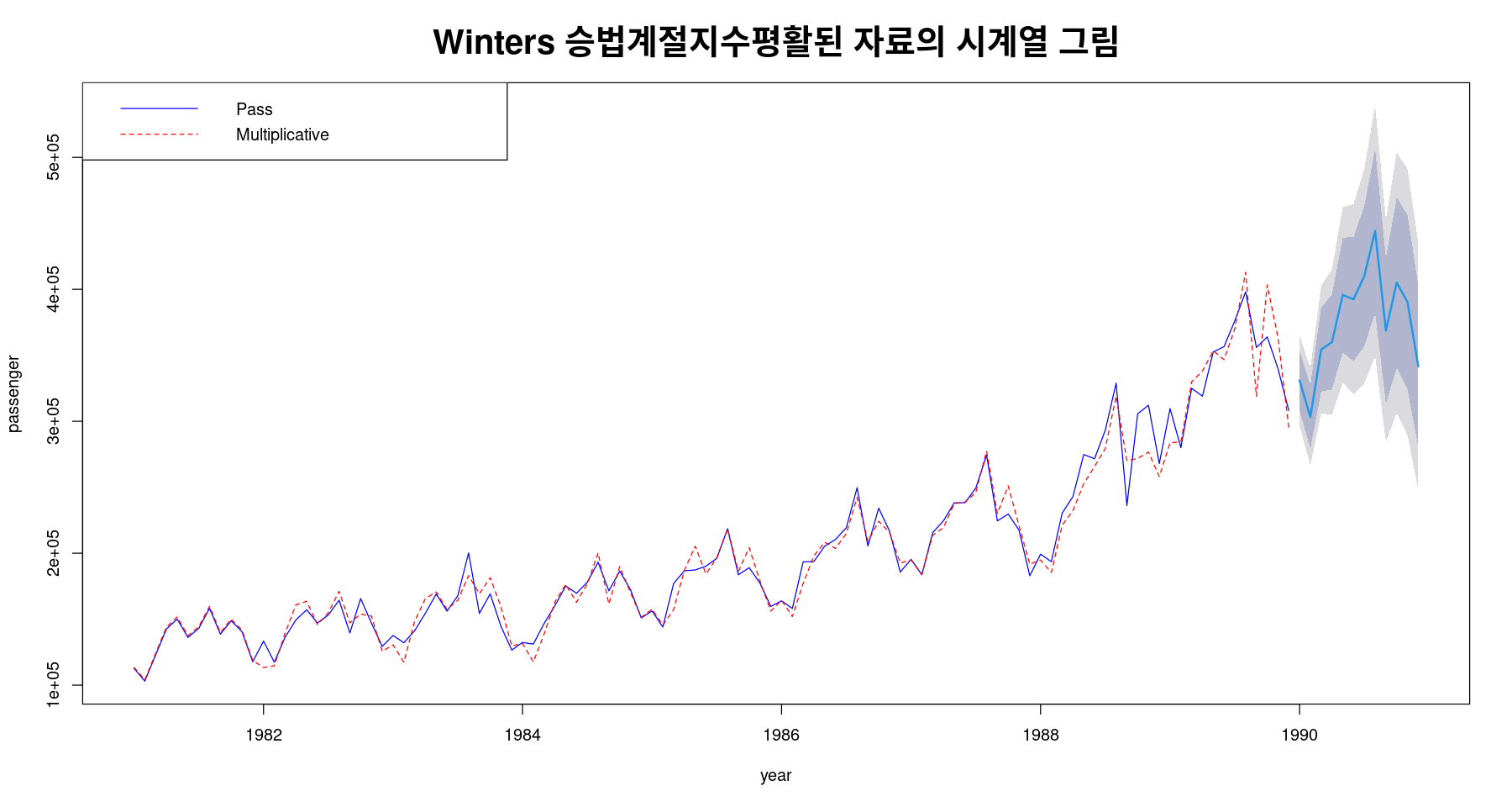
ts.plot(fit7$residual, ylab="residual",
 main="승법모형의 잔차 그림",
 cex.main=2); abline(h=0)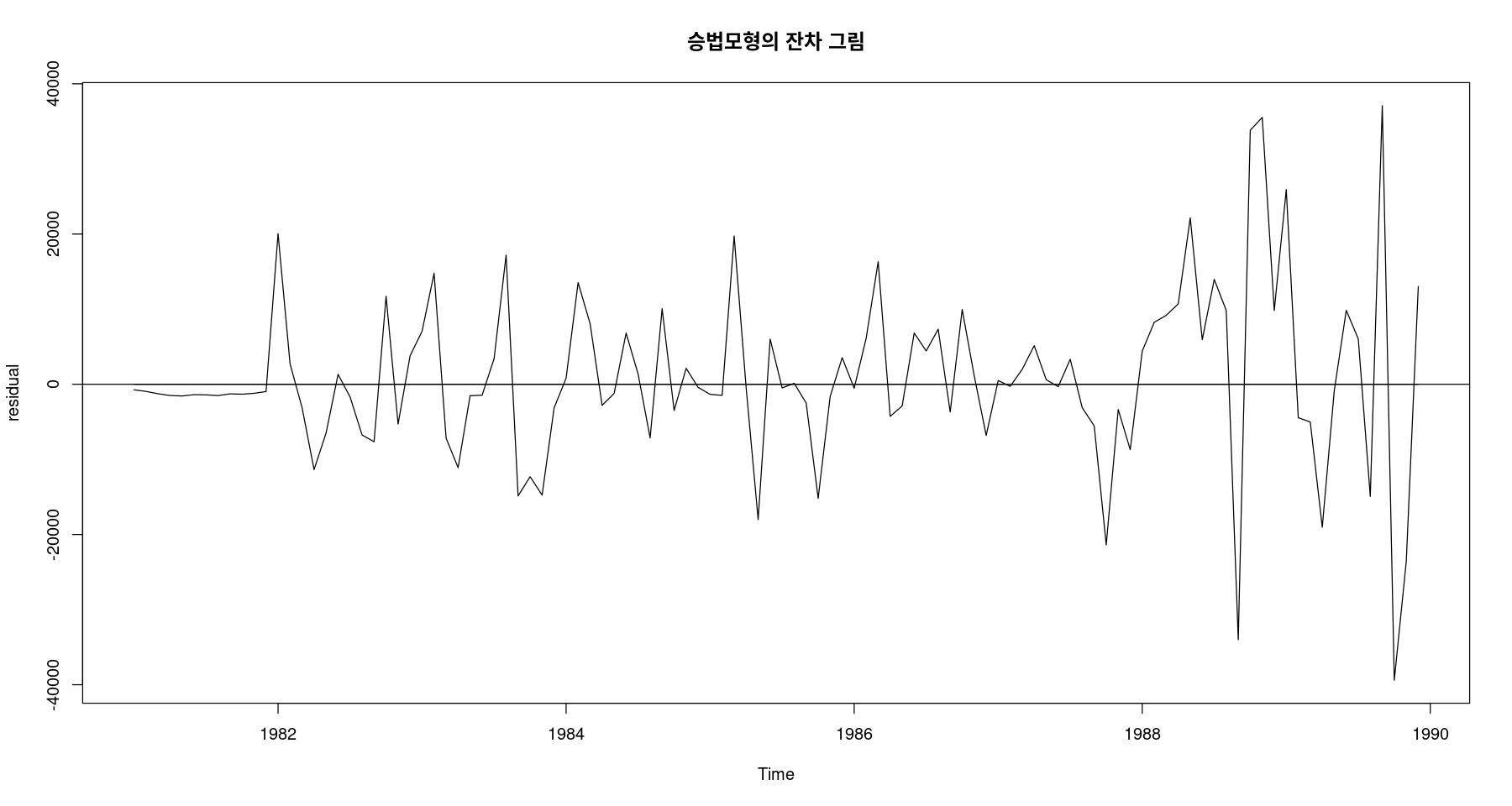
dwtest(lm(fit7$residual~1), alternative = 'two.sided')
    Durbin-Watson test

data:  lm(fit7$residual ~ 1)
DW = 1.9744, p-value = 0.8931
alternative hypothesis: true autocorrelation is not 0fit_hw$SSEfit_hw_m$SSE가법과 승법 모형의 SSE를 비교해서 SSE값이 더 작은 모형을 선택해 주자.
단순지수평활: HoltWinters(beta=gamma=FALSE), ses: 추세도 없고 계절성분도 없어보일 때 사용
이중지수평활: HoltWinters(gamma=FALSE), holt: 추세가 있을 때 사용
계절지수평활: HoltWinters(), hw: 계절 성분 있을 때 사용
위의 함수를 사용하기 전에 가장 먼저 시도표를 보자!